Methods
This page describes how we selected representative specimens and obtained sequences for three regions of mitochondrial DNA (cytochrome oxidase I [COI], cytochrome b [CytB], and the control region [D-loop]. We then estimated a reference phylogeny and identified phylogenetic clades, which we relabeled as operational phylogenetic species. These clades form the basis of our system of identification. This work is described in Robins et al. (2007).Samples
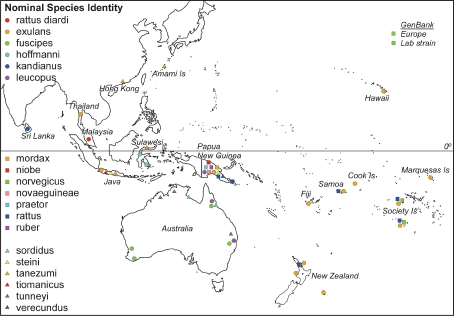
Of the 118 samples in our analysis, three were complete mitochondrial genome sequences from R. norvegicus obtained from GenBank, two of which were from laboratory strains and the third was caught in the wild in Denmark. Of the remaining samples, 94 were tissues obtained from the South Australian Museum and bore the names given by the museum, and 21 were from rats trapped in the field by one of us (EM-S) and identified using Cunningham and Moors (1983). The geographical distribution of the samples were: 21 R. exulans from Thailand, New Guinea and the Pacific, 5 R. fuscipes from Australia, 3 R. hoffmanni from Sulawesi, 3 R. kandianus from Sri Lanka, 6 R. leucopus from New Guinea and Australia, 1 R. mordax from New Guinea, 6 R. niobe from New Guinea, 2 R. norvegicus from the Society Islands, 1 R. novaeguineae from New Guinea, 6 R. praetor from New Guinea, 7 R. rattus from New Guinea and across the Pacific, 5 R. rattus diardi (not diardii ) from Malaysia, 1 R. ruber from New Guinea, 4 R. sordidus from Australia, 9 R. steini from Indonesia and New Guinea, 24 R. tanezumi from Japan, Hong Kong and Indonesia, 2 R. tiomanicus from Indonesia, 4 R. tunneyi from Australia, and 5 R. verecundus from New Guinea. Sample locations of the Rattus species included in this study. For locations with many different species sampled (e.g., Java and Papua New Guinea) the positions indicated are not informative.
Sequencing
Rat tissues were stored in 70% ethanol and DNA was extracted from them using either standard phenol chloroform methods (Sambrook et al., 1989) or the High Pure PCR Template Preparation Kit from Roche. The amplification reactions contained: TrisHCl pH 8.3 10 mM; KCl 50 mM; forward and reverse primers at 0.5M each; dNTPs at 0.15mM each; 0.5 units of Taq polymerase; 1L of DNA template.To amplify 750 bp of COI, the primers used were:
- BatL5310 (5-CCTACTCRGCCATTTTACCTATG-3), and
- R6036R (5-ACTTCTGGGTGTCCAAAGAATCA-3);
- RGlu2L (5-CAGCATTTAACTGTGACTAATGAC-3) and
- RCb9H (5-TACACCTAGGAGGTCTTTAATTG-3); and
- EGL4L (5-CCACCATCAACACCCAAAG-3) and
- RJ3R (5-CATGCCTTGACGGCTATGTTG-3).
The sequences for each region were aligned in Sequencher, adjusted manually and then trimmed to a common length (D-loop 535 bp, cytochrome b 713 bp, COI 702 bp).
Tree building
The phylogenetic relationships among the samples was inferred from a Bayesian partitioned likelihood analysis (MrBayes v3.1, Huelsenbeck, Ronquist, 2001) of the concatenated sequences. Each genomic region was treated as a separate data partition. The GTR+G model of evolution was used with parameters unlinked across partitions to give slightly greater parameterisation than was indicated by ModelTest (below) for each region. The analysis was run on 4 chains (temperature = 0.2) for 12 million generations, with trees sampled every 1000 generations. After visual inspection, the first 100 trees (100,000 generations) were discarded and a 50% consensus tree was constructed from the remaining trees. The analysis was run twice, with different randomly chosen starting trees. The phylogeny was also checked by using maximum likelihood (PHYML, Guindon, Gascuel, 2003) to infer a phylogenetic tree separately for each genomic region, using the HKY+I+G model of evolution and estimated model parameter values as identified by ModelTest (Posada, Crandall, 1998). Clade support was estimated with 100 bootstrap replicates for eachregion.
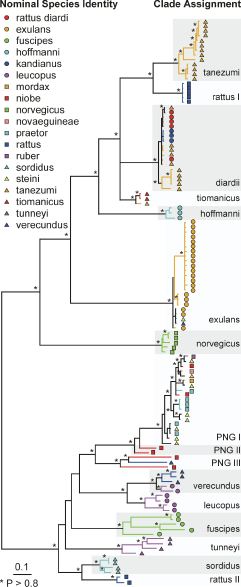
Phylogeny of the Rattus specimens estimated using Bayesian partitioned likelihood. Nodes with posterior P >0.8 are marked by *. The nominal species identity of individual specimens is indicated by a combination of symbol shape and colour. Clades indicated by alternating grey or white bands are named operationally as phylogenetic species. The tree has been rooted using Mus musculus (not shown).
Reference Datasets
From the specimens listed in the map and tree above, a subset was chosen for use as reference sequences in DNA Surveillance. The specimens were selected so as to provide representative coverage of all of the clades, to the extent possible.Below is a list of the current reference datasets available, with links to more information.
| Domain | Cytochrome Oxidase I (v2) = COI_v2 | Cytochrome b (v2) = CytB_v2 | Control Region (v2) = DLoop_v2 | Cytochrome Oxidase I (v3) = COI_v3 | Cytochrome b (v3) = CytB_v3 | Control Region (v3) = DLoop_v3 |
|---|---|---|---|---|---|---|
| Rattus | Link | Link | Link | Link | Link | Link |
| Pos 1-250 | N/A | N/A | N/A | N/A | N/A | Link |
| Pos 1-200 | N/A | N/A | N/A | Link | N/A | N/A |
| Pos 101-300 | N/A | N/A | N/A | Link | N/A | N/A |
| Pos 201-400 | N/A | N/A | N/A | Link | N/A | N/A |
| Pos 301-500 | N/A | N/A | N/A | Link | N/A | N/A |
| Pos 401-600 | N/A | N/A | N/A | Link | N/A | N/A |
| Pos 501-end | N/A | N/A | N/A | Link | N/A | N/A |
Species identification
Two approaches to species identification are possible:- Construct a neighbor-joining (NJ) tree using your submitted query sequence and the corresponding reference sequences. The genetic distances are estimated using the parameter values given with the details of the reference datasets. The entire tree is re-estimated in each analysis.
- Estimate the maximum likelihood placement of your submitted query sequence on the appropriate reference topology. For each gene region (COI, cytochrome b, D-loop), we have estimated a maximum likelihood tree from the reference sequences and uploaded it as a reference topology.
References
- Cunningham D, Moors P (1983) A Guide to the Identification and Collection of New Zealand Rodents, Edition edn. Department of Internal Affairs, Wellington, New Zealand.
- Felsenstein, J. 1984 Distance methods for inferring phylogenies: A justification. Evolution 38, 16-24.
- Guindon S, Gascuel O (2003) A simple,fast, and accurate algorithm to estimate large phylogenies by maximum likelihood. Systematic Biology 52, 696-704.
- Gribskov, M., Luthy, R. Eisenberg, D. (1990) Profile analysis. Methods in Enzymology 183, 146-159.
- Gribskov, M., McLachlan, A. D. Eisenberg, D. (1987) Profile analysis: detection of distantly related proteins. Proceedings of the National Academy of Science of the USA 84, 4355-4358.
- Huelsenbeck JP, Ronquist F (2001) MRBAYES: Bayesian inference of phylogeny. Bioinformatics 17, 754-755.
- Kishino, H. and Hasegawa, M. 1989 Evaluation of the maximum likelihood estimate of the evolutionary tree topologies from DNA sequence data, and the branching order in Hominoidea. Journal of Molecular Evolution 29, 170-179.
- Posada D, Crandall K (1998) MODELTEST: testing the model of DNA substitution. Bioinformatics 14, 817-818.
- Robins JH, Hingston M, Matisoo-Smith E, Ross H (2007) Identifying Rattus species using mitochondrial DNA. Molecular Ecology Notes 7:717-729.
- Saitou, N. and Nei, M. 1987 The neighbor-joining method: A new method for reconstructing phylogenetic trees. Molecular Biology and Evolution 4, 406-425.
- Sambrook J, Fritsch EF, Maniatis T (1989) Molecular cloning: a laboratory manual, 2nd edn., Cold Spring Harbour Laboratory, Cold Spring Harbor.
- Thompson, J. D., Gibson, T. J., Plewniak, F., Jeanmougin, F. Higgins, D. G. (1997) The ClustalX windows interface: flexible strategies for multiple sequence alignment aided by quality analysis tools. Nucleic Acids Research 24, 4876-4882.
